目錄
- 一、前言
- 二、Blending介紹
- 三、Blending流程圖
- 四、案例
一、前言
普通機器學習:從訓練數據中學習一個假設。
集成方法:試圖構建一組假設并將它們組合起來,集成學習是一種機器學習范式,多個學習器被訓練來解決同一個問題。
集成方法分類為:
Bagging(并行訓練):隨機森林
Boosting(串行訓練):Adaboost; GBDT; XgBoost
Stacking:
Blending:
或者分類為串行集成方法和并行集成方法
1.串行模型:通過基礎模型之間的依賴,給錯誤分類樣本一個較大的權重來提升模型的性能。
2.并行模型的原理:利用基礎模型的獨立性,然后通過平均能夠較大地降低誤差
二、Blending介紹
訓練數據劃分為訓練和驗證集+新的訓練數據集和新的測試集
將訓練數據進行劃分,劃分之后的訓練數據一部分訓練基模型,一部分經模型預測后作為新的特征訓練元模型。
測試數據同樣經過基模型預測,形成新的測試數據。最后,元模型對新的測試數據進行預測。Blending框架圖如下所示:
注意:其是在stacking的基礎上加了劃分數據
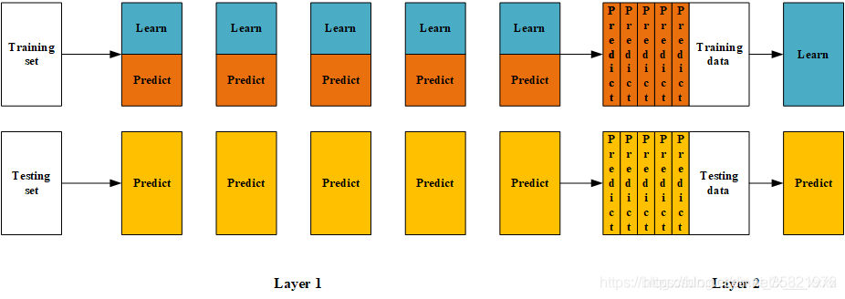
三、Blending流程圖
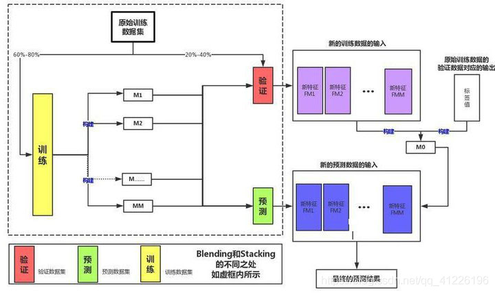
- 第一步:將原始訓練數據劃分為訓練集和驗證集。
- 第二步:使用訓練集對訓練T個不同的模型。
- 第三步:使用T個基模型,對驗證集進行預測,結果作為新的訓練數據。
- 第四步:使用新的訓練數據,訓練一個元模型。
- 第五步:使用T個基模型,對測試數據進行預測,結果作為新的測試數據。
- 第六步:使用元模型對新的測試數據進行預測,得到最終結果。
四、案例
相關工具包加載
import numpy as np
import pandas as pd
import matplotlib.pyplot as plt
plt.style.use("ggplot")
%matplotlib inline
import seaborn as sns
創建數據
from sklearn import datasets
from sklearn.datasets import make_blobs
from sklearn.model_selection import train_test_split
data, target = make_blobs(n_samples=10000, centers=2, random_state=1, cluster_std=1.0 )
## 創建訓練集和測試集
X_train1,X_test,y_train1,y_test = train_test_split(data, target, test_size=0.2, random_state=1)
## 創建訓練集和驗證集
X_train,X_val,y_train,y_val = train_test_split(X_train1, y_train1, test_size=0.3, random_state=1)
print("The shape of training X:",X_train.shape)
print("The shape of training y:",y_train.shape)
print("The shape of test X:",X_test.shape)
print("The shape of test y:",y_test.shape)
print("The shape of validation X:",X_val.shape)
print("The shape of validation y:",y_val.shape)
設置第一層分類器
from sklearn.svm import SVC
from sklearn.ensemble import RandomForestClassifier
from sklearn.neighbors import KNeighborsClassifier
clfs = [SVC(probability=True),RandomForestClassifier(n_estimators=5,n_jobs=-1,criterion='gini'),KNeighborsClassifier()]
設置第二層分類器
from sklearn.linear_model import LinearRegression
lr = LinearRegression()
第一層
val_features = np.zeros((X_val.shape[0],len(clfs)))
test_features = np.zeros((X_test.shape[0],len(clfs)))
for i,clf in enumerate(clfs):
    clf.fit(X_train,y_train)
    val_feature = clf.predict_proba(X_val)[:,1]
    test_feature = clf.predict_proba(X_test)[:,1]
    val_features[:,i] = val_feature
    test_features[:,i] = test_feature
第二層
lr.fit(val_features,y_val)
輸出預測的結果
lr.fit(val_features,y_val)
from sklearn.model_selection import cross_val_score
cross_val_score(lr,test_features,y_test,cv=5)
到此這篇關于Python集成學習之Blending算法詳解的文章就介紹到這了,更多相關Python Blending算法內容請搜索腳本之家以前的文章或繼續瀏覽下面的相關文章希望大家以后多多支持腳本之家!
您可能感興趣的文章:- python 算法題——快樂數的多種解法
- python使用ProjectQ生成量子算法指令集
- Python機器學習算法之決策樹算法的實現與優缺點
- python3實現Dijkstra算法最短路徑的實現
- Python實現K-means聚類算法并可視化生成動圖步驟詳解
- Python自然語言處理之切分算法詳解
- python入門之算法學習
- Python實現機器學習算法的分類