1717she国产精品成年,国产成人啪精品视频免费软件

技術(shù)背景

在數(shù)學(xué)和物理學(xué)領(lǐng)域，總是充滿了各種連續(xù)的函數(shù)模型。而當(dāng)我們用現(xiàn)代計(jì)算機(jī)的技術(shù)去處理這些問題的時(shí)候，事實(shí)上是無法直接處理連續(xù)模型的，絕大多數(shù)的情況下都要轉(zhuǎn)化成一個離散的模型再進(jìn)行數(shù)值的計(jì)算。比如計(jì)算數(shù)值的積分，計(jì)算數(shù)值的二階導(dǎo)數(shù)（海森矩陣）等等。這里我們所介紹的打格點(diǎn)的算法，正是一種典型的離散化方法。這個對空間做離散化的方法，可以在很大程度上簡化運(yùn)算量。比如在分子動力學(xué)模擬中，計(jì)算近鄰表的時(shí)候，如果不采用打格點(diǎn)的方法，那么就要針對整個空間所有的原子進(jìn)行搜索，計(jì)算出來距離再判斷是否近鄰。而如果采用打格點(diǎn)的方法，我們只需要先遍歷一遍原子對齊進(jìn)行打格點(diǎn)的離散化，之后再計(jì)算近鄰表的時(shí)候，只需要計(jì)算三維空間下鄰近的27個格子中的原子是否滿足近鄰條件即可。在這篇文章中，我們主要探討如何用GPU來實(shí)現(xiàn)打格點(diǎn)的算法。

打格點(diǎn)算法實(shí)現(xiàn)

我們先來用一個例子說明一下什么叫打格點(diǎn)。對于一個給定所有原子坐標(biāo)的系統(tǒng)，也就是已知了[x,y,z]，我們需要得到的是這些原子所在的對應(yīng)的格子位置[n_x,n_y,n_z]。我們先看一下在CPU上的實(shí)現(xiàn)方案，是一個遍歷一次的算法：

# cuda_grid.py

from numba import jit
from numba import cuda
import numpy as np

def grid_by_cpu(crd, rxyz, atoms, grids):
    """Transform coordinates [x,y,z] into grids [nx,ny,nz].
    Args:
        crd(list): The 3-D coordinates of atoms.
        rxyz(list): The list includes xmin,ymin,zmin,grid_num.
        atoms(int): The total number of atoms.
        grids(list): The transformed grids matrix.
    """
    for i in range(atoms):
        grids[i][0] = int((crd[i][0]-rxyz[0])/rxyz[3])
        grids[i][1] = int((crd[i][1]-rxyz[1])/rxyz[3])
        grids[i][2] = int((crd[i][2]-rxyz[2])/rxyz[3])
    return grids

if __name__=='__main__':
    np.random.seed(1)
    atoms = 4
    grid_size = 0.1
    crd = np.random.random((atoms,3)).astype(np.float32)
    xmin = min(crd[:,0])
    ymin = min(crd[:,1])
    zmin = min(crd[:,2])
    xmax = max(crd[:,0])
    ymax = max(crd[:,1])
    zmax = max(crd[:,2])
    xgrids = int((xmax-xmin)/grid_size)+1
    ygrids = int((ymax-ymin)/grid_size)+1
    zgrids = int((zmax-zmin)/grid_size)+1
    rxyz = np.array([xmin,ymin,zmin,grid_size], dtype=np.float32)
    
    grids = np.ones_like(crd)*(-1)
    grids = grids.astype(np.float32)
    grids_cpu = grid_by_cpu(crd, rxyz, atoms, grids)
    print (crd)
    print (grids_cpu)

    import matplotlib.pyplot as plt
    plt.figure()
    plt.plot(crd[:,0], crd[:,1], 'o', color='red')
    for grid in range(ygrids+1):
        plt.plot([xmin,xmin+grid_size*xgrids], [ymin+grid_size*grid,ymin+grid_size*grid], color='black')
    for grid in range(xgrids+1):
        plt.plot([xmin+grid_size*grid,xmin+grid_size*grid], [ymin,ymin+grid_size*ygrids], color='black')
    plt.savefig('Atom_Grids.png')

輸出結(jié)果如下，

$ python3 cuda_grid.py
[[4.17021990e-01 7.20324516e-01 1.14374816e-04]
[3.02332580e-01 1.46755889e-01 9.23385918e-02]
[1.86260208e-01 3.45560730e-01 3.96767467e-01]
[5.38816750e-01 4.19194520e-01 6.85219526e-01]]
[[2. 5. 0.]
[1. 0. 0.]
[0. 1. 3.]
[3. 2. 6.]]

上面兩個打印輸出就分別對應(yīng)于[x,y,z]和[nx,ny,nz]，比如第一個原子被放到了編號為[2,5,0]的格點(diǎn)。那么為了方便理解打格點(diǎn)的方法，我們把這個三維空間的原子系統(tǒng)和打格點(diǎn)以后的標(biāo)號取前兩個維度來可視化一下結(jié)果，作圖以后效果如下：

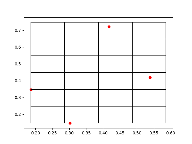
我們可以看到，這些紅色的點(diǎn)就是原子所處的位置，而黑色的網(wǎng)格線就是我們所標(biāo)記的格點(diǎn)。在原子數(shù)量比較多的時(shí)候，有可能出現(xiàn)在一個網(wǎng)格中存在很多個原子的情況，所以如何打格點(diǎn)，格點(diǎn)大小如何去定義，這都是不同場景下的經(jīng)驗(yàn)參數(shù)，需要大家一起去摸索。

打格點(diǎn)算法加速

在上面這個算法實(shí)現(xiàn)中，我們主要是用到了一個for循環(huán)，這時(shí)候我們可以想到numba所支持的向量化運(yùn)算，還有GPU硬件加速，這里我們先對比一下三種實(shí)現(xiàn)方案的計(jì)算結(jié)果：

# cuda_grid.py

from numba import jit
from numba import cuda
import numpy as np

def grid_by_cpu(crd, rxyz, atoms, grids):
    """Transform coordinates [x,y,z] into grids [nx,ny,nz].
    Args:
        crd(list): The 3-D coordinates of atoms.
        rxyz(list): The list includes xmin,ymin,zmin,grid_num.
        atoms(int): The total number of atoms.
        grids(list): The transformed grids matrix.
    """
    for i in range(atoms):
        grids[i][0] = int((crd[i][0]-rxyz[0])/rxyz[3])
        grids[i][1] = int((crd[i][1]-rxyz[1])/rxyz[3])
        grids[i][2] = int((crd[i][2]-rxyz[2])/rxyz[3])
    return grids

@jit
def grid_by_jit(crd, rxyz, atoms, grids):
    """Transform coordinates [x,y,z] into grids [nx,ny,nz].
    Args:
        crd(list): The 3-D coordinates of atoms.
        rxyz(list): The list includes xmin,ymin,zmin,grid_num.
        atoms(int): The total number of atoms.
        grids(list): The transformed grids matrix.
    """
    for i in range(atoms):
        grids[i][0] = int((crd[i][0]-rxyz[0])/rxyz[3])
        grids[i][1] = int((crd[i][1]-rxyz[1])/rxyz[3])
        grids[i][2] = int((crd[i][2]-rxyz[2])/rxyz[3])
    return grids

@cuda.jit
def grid_by_gpu(crd, rxyz, grids):
    """Transform coordinates [x,y,z] into grids [nx,ny,nz].
    Args:
        crd(list): The 3-D coordinates of atoms.
        rxyz(list): The list includes xmin,ymin,zmin,grid_num.
        atoms(int): The total number of atoms.
        grids(list): The transformed grids matrix.
    """
    i,j = cuda.grid(2)
    grids[i][j] = int((crd[i][j]-rxyz[j])/rxyz[3])

if __name__=='__main__':
    np.random.seed(1)
    atoms = 4
    grid_size = 0.1
    crd = np.random.random((atoms,3)).astype(np.float32)
    xmin = min(crd[:,0])
    ymin = min(crd[:,1])
    zmin = min(crd[:,2])
    xmax = max(crd[:,0])
    ymax = max(crd[:,1])
    zmax = max(crd[:,2])
    xgrids = int((xmax-xmin)/grid_size)+1
    ygrids = int((ymax-ymin)/grid_size)+1
    zgrids = int((zmax-zmin)/grid_size)+1
    rxyz = np.array([xmin,ymin,zmin,grid_size], dtype=np.float32)
    crd_cuda = cuda.to_device(crd)
    rxyz_cuda = cuda.to_device(rxyz)
    
    grids = np.ones_like(crd)*(-1)
    grids = grids.astype(np.float32)
    grids_cpu = grid_by_cpu(crd, rxyz, atoms, grids)

    grids = np.ones_like(crd)*(-1)
    grids_jit = grid_by_jit(crd, rxyz, atoms, grids)

    grids = np.ones_like(crd)*(-1)
    grids_cuda = cuda.to_device(grids)
    
    grid_by_gpu[(atoms,3),(1,1)](crd_cuda,
                                 rxyz_cuda,
                                 grids_cuda)

    print (crd)
    print (grids_cpu)
    print (grids_jit)
    print (grids_cuda.copy_to_host())

輸出結(jié)果如下：

$ python3 cuda_grid.py
/home/dechin/anaconda3/lib/python3.8/site-packages/numba/cuda/compiler.py:865: NumbaPerformanceWarning: Grid size (12) 2 * SM count (72) will likely result in GPU under utilization due to low occupancy.
warn(NumbaPerformanceWarning(msg))
[[4.17021990e-01 7.20324516e-01 1.14374816e-04]
[3.02332580e-01 1.46755889e-01 9.23385918e-02]
[1.86260208e-01 3.45560730e-01 3.96767467e-01]
[5.38816750e-01 4.19194520e-01 6.85219526e-01]]
[[2. 5. 0.]
[1. 0. 0.]
[0. 1. 3.]
[3. 2. 6.]]
[[2. 5. 0.]
[1. 0. 0.]
[0. 1. 3.]
[3. 2. 6.]]
[[2. 5. 0.]
[1. 0. 0.]
[0. 1. 3.]
[3. 2. 6.]]

我們先看到這里面的告警信息，因?yàn)镚PU硬件加速要在一定密度的運(yùn)算量之上才能夠有比較明顯的加速效果。比如說我們只是計(jì)算兩個數(shù)字的加和，那么是完全沒有必要使用到GPU的。但是如果我們要計(jì)算兩個非常大的數(shù)組的加和，那么這個時(shí)候GPU就能夠發(fā)揮出非常大的價(jià)值。因?yàn)檫@里我們的案例中只有4個原子，因此提示我們這時(shí)候是體現(xiàn)不出來GPU的加速效果的。我們僅僅關(guān)注下這里的運(yùn)算結(jié)果，在不同體系下得到的格點(diǎn)結(jié)果是一致的，那么接下來就可以對比一下幾種不同實(shí)現(xiàn)方式的速度差異。

# cuda_grid.py

from numba import jit
from numba import cuda
import numpy as np

def grid_by_cpu(crd, rxyz, atoms, grids):
    """Transform coordinates [x,y,z] into grids [nx,ny,nz].
    Args:
        crd(list): The 3-D coordinates of atoms.
        rxyz(list): The list includes xmin,ymin,zmin,grid_num.
        atoms(int): The total number of atoms.
        grids(list): The transformed grids matrix.
    """
    for i in range(atoms):
        grids[i][0] = int((crd[i][0]-rxyz[0])/rxyz[3])
        grids[i][1] = int((crd[i][1]-rxyz[1])/rxyz[3])
        grids[i][2] = int((crd[i][2]-rxyz[2])/rxyz[3])
    return grids

@jit
def grid_by_jit(crd, rxyz, atoms, grids):
    """Transform coordinates [x,y,z] into grids [nx,ny,nz].
    Args:
        crd(list): The 3-D coordinates of atoms.
        rxyz(list): The list includes xmin,ymin,zmin,grid_num.
        atoms(int): The total number of atoms.
        grids(list): The transformed grids matrix.
    """
    for i in range(atoms):
        grids[i][0] = int((crd[i][0]-rxyz[0])/rxyz[3])
        grids[i][1] = int((crd[i][1]-rxyz[1])/rxyz[3])
        grids[i][2] = int((crd[i][2]-rxyz[2])/rxyz[3])
    return grids

@cuda.jit
def grid_by_gpu(crd, rxyz, grids):
    """Transform coordinates [x,y,z] into grids [nx,ny,nz].
    Args:
        crd(list): The 3-D coordinates of atoms.
        rxyz(list): The list includes xmin,ymin,zmin,grid_num.
        atoms(int): The total number of atoms.
        grids(list): The transformed grids matrix.
    """
    i,j = cuda.grid(2)
    grids[i][j] = int((crd[i][j]-rxyz[j])/rxyz[3])

if __name__=='__main__':
    import time
    from tqdm import trange

    np.random.seed(1)
    atoms = 100000
    grid_size = 0.1
    crd = np.random.random((atoms,3)).astype(np.float32)
    xmin = min(crd[:,0])
    ymin = min(crd[:,1])
    zmin = min(crd[:,2])
    xmax = max(crd[:,0])
    ymax = max(crd[:,1])
    zmax = max(crd[:,2])
    xgrids = int((xmax-xmin)/grid_size)+1
    ygrids = int((ymax-ymin)/grid_size)+1
    zgrids = int((zmax-zmin)/grid_size)+1
    rxyz = np.array([xmin,ymin,zmin,grid_size], dtype=np.float32)
    crd_cuda = cuda.to_device(crd)
    rxyz_cuda = cuda.to_device(rxyz)
    
    cpu_time = 0
    jit_time = 0
    gpu_time = 0

    for i in trange(100):
        grids = np.ones_like(crd)*(-1)
        grids = grids.astype(np.float32)
        time0 = time.time()
        grids_cpu = grid_by_cpu(crd, rxyz, atoms, grids)
        time1 = time.time()

        grids = np.ones_like(crd)*(-1)
        time2 = time.time()
        grids_jit = grid_by_jit(crd, rxyz, atoms, grids)
        time3 = time.time()

        grids = np.ones_like(crd)*(-1)
        grids_cuda = cuda.to_device(grids)
        time4 = time.time()
        grid_by_gpu[(atoms,3),(1,1)](crd_cuda,
                                    rxyz_cuda,
                                    grids_cuda)
        time5 = time.time()
        
        if i != 0:
            cpu_time += time1 - time0
            jit_time += time3 - time2
            gpu_time += time5 - time4
    
    print ('The time cost of CPU calculation is: {}s'.format(cpu_time))
    print ('The time cost of JIT calculation is: {}s'.format(jit_time))
    print ('The time cost of GPU calculation is: {}s'.format(gpu_time))

輸出結(jié)果如下：

$ python3 cuda_grid.py
100%|███████████████████████████| 100/100 [00:2300:00, 4.18it/s]
The time cost of CPU calculation is: 23.01943016052246s
The time cost of JIT calculation is: 0.04810166358947754s
The time cost of GPU calculation is: 0.01806473731994629s

在100000個原子的體系規(guī)模下，普通的for循環(huán)實(shí)現(xiàn)效率就非常的低下，需要23s，而經(jīng)過向量化運(yùn)算的加速之后，直接飛升到了0.048s，而GPU上的加速更是達(dá)到了0.018s，相比于沒有GPU硬件加速的場景，實(shí)現(xiàn)了將近2倍的加速。但是這還遠(yuǎn)遠(yuǎn)不是GPU加速的上限，讓我們再測試一個更大的案例：

# cuda_grid.py

from numba import jit
from numba import cuda
import numpy as np

def grid_by_cpu(crd, rxyz, atoms, grids):
    """Transform coordinates [x,y,z] into grids [nx,ny,nz].
    Args:
        crd(list): The 3-D coordinates of atoms.
        rxyz(list): The list includes xmin,ymin,zmin,grid_num.
        atoms(int): The total number of atoms.
        grids(list): The transformed grids matrix.
    """
    for i in range(atoms):
        grids[i][0] = int((crd[i][0]-rxyz[0])/rxyz[3])
        grids[i][1] = int((crd[i][1]-rxyz[1])/rxyz[3])
        grids[i][2] = int((crd[i][2]-rxyz[2])/rxyz[3])
    return grids

@jit
def grid_by_jit(crd, rxyz, atoms, grids):
    """Transform coordinates [x,y,z] into grids [nx,ny,nz].
    Args:
        crd(list): The 3-D coordinates of atoms.
        rxyz(list): The list includes xmin,ymin,zmin,grid_num.
        atoms(int): The total number of atoms.
        grids(list): The transformed grids matrix.
    """
    for i in range(atoms):
        grids[i][0] = int((crd[i][0]-rxyz[0])/rxyz[3])
        grids[i][1] = int((crd[i][1]-rxyz[1])/rxyz[3])
        grids[i][2] = int((crd[i][2]-rxyz[2])/rxyz[3])
    return grids

@cuda.jit
def grid_by_gpu(crd, rxyz, grids):
    """Transform coordinates [x,y,z] into grids [nx,ny,nz].
    Args:
        crd(list): The 3-D coordinates of atoms.
        rxyz(list): The list includes xmin,ymin,zmin,grid_num.
        atoms(int): The total number of atoms.
        grids(list): The transformed grids matrix.
    """
    i,j = cuda.grid(2)
    grids[i][j] = int((crd[i][j]-rxyz[j])/rxyz[3])

if __name__=='__main__':
    import time
    from tqdm import trange

    np.random.seed(1)
    atoms = 5000000
    grid_size = 0.1
    crd = np.random.random((atoms,3)).astype(np.float32)
    xmin = min(crd[:,0])
    ymin = min(crd[:,1])
    zmin = min(crd[:,2])
    xmax = max(crd[:,0])
    ymax = max(crd[:,1])
    zmax = max(crd[:,2])
    xgrids = int((xmax-xmin)/grid_size)+1
    ygrids = int((ymax-ymin)/grid_size)+1
    zgrids = int((zmax-zmin)/grid_size)+1
    rxyz = np.array([xmin,ymin,zmin,grid_size], dtype=np.float32)
    crd_cuda = cuda.to_device(crd)
    rxyz_cuda = cuda.to_device(rxyz)

    jit_time = 0
    gpu_time = 0

    for i in trange(100):
        grids = np.ones_like(crd)*(-1)
        time2 = time.time()
        grids_jit = grid_by_jit(crd, rxyz, atoms, grids)
        time3 = time.time()

        grids = np.ones_like(crd)*(-1)
        grids_cuda = cuda.to_device(grids)
        time4 = time.time()
        grid_by_gpu[(atoms,3),(1,1)](crd_cuda,
                                     rxyz_cuda,
                                     grids_cuda)
        time5 = time.time()
        
        if i != 0:
            jit_time += time3 - time2
            gpu_time += time5 - time4
    
    print ('The time cost of JIT calculation is: {}s'.format(jit_time))
    print ('The time cost of GPU calculation is: {}s'.format(gpu_time))

在這個5000000個原子的案例中，因?yàn)槠胀ǖ膄or循環(huán)已經(jīng)實(shí)在是跑不動了，因此我們就干脆不統(tǒng)計(jì)這一部分的時(shí)間，最后輸出結(jié)果如下：

$ python3 cuda_grid.py
100%|███████████████████████████| 100/100 [00:0900:00, 10.15it/s]
The time cost of JIT calculation is: 2.3743042945861816s
The time cost of GPU calculation is: 0.022843599319458008s

在如此大規(guī)模的運(yùn)算下，GPU實(shí)現(xiàn)100倍的加速，而此時(shí)作為對比的CPU上的實(shí)現(xiàn)方法是已經(jīng)用上了向量化運(yùn)算的操作，也已經(jīng)可以認(rèn)為是一個極致的加速了。

總結(jié)概要

在這篇文章中，我們主要介紹了打格點(diǎn)算法在分子動力學(xué)模擬中的重要價(jià)值，以及幾種不同的實(shí)現(xiàn)方式。其中最普通的for循環(huán)的實(shí)現(xiàn)效率比較低下，從算法復(fù)雜度上來講卻已經(jīng)是極致。而基于CPU上的向量化運(yùn)算的技術(shù)，可以對計(jì)算過程進(jìn)行非常深度的優(yōu)化。當(dāng)然，這個案例在不同的硬件上也能夠發(fā)揮出明顯不同的加速效果，在GPU的加持之下，可以獲得100倍以上的加速效果。這也是一個在Python上實(shí)現(xiàn)GPU加速算法的一個典型案例。

到此這篇關(guān)于Python3實(shí)現(xiàn)打格點(diǎn)算法的GPU加速的文章就介紹到這了,更多相關(guān)Python3實(shí)現(xiàn)打格點(diǎn)算法內(nèi)容請搜索腳本之家以前的文章或繼續(xù)瀏覽下面的相關(guān)文章希望大家以后多多支持腳本之家！

您可能感興趣的文章:

Python3爬樓梯算法示例
Python3 A*尋路算法實(shí)現(xiàn)方式
Python3.0 實(shí)現(xiàn)決策樹算法的流程
Python3實(shí)現(xiàn)的判斷環(huán)形鏈表算法示例

標(biāo)簽：吉安安康懷化蘭州蕪湖紹興呂梁廣西

巨人網(wǎng)絡(luò)通訊聲明：本文標(biāo)題《Python3實(shí)現(xiàn)打格點(diǎn)算法的GPU加速實(shí)例詳解》，本文關(guān)鍵詞 Python3,實(shí)現(xiàn),打格點(diǎn),算法,；如發(fā)現(xiàn)本文內(nèi)容存在版權(quán)問題，煩請?zhí)峁┫嚓P(guān)信息告之我們，我們將及時(shí)溝通與處理。本站內(nèi)容系統(tǒng)采集于網(wǎng)絡(luò)，涉及言論、版權(quán)與本站無關(guān)。