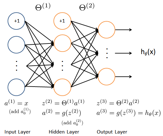
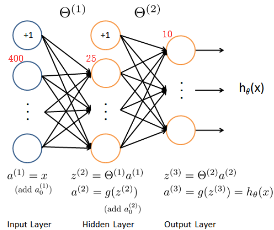
1 Neural Networks 神經網絡
1.1 Visualizing the data 可視化數據
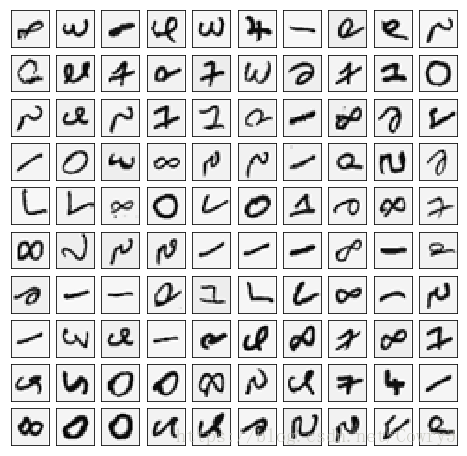
這部分我們隨機選取100個樣本并可視化。訓練集共有5000個訓練樣本,每個樣本是20*20像素的數字的灰度圖像。每個像素代表一個浮點數,表示該位置的灰度強度。20×20的像素網格被展開成一個400維的向量。在我們的數據矩陣X中,每一個樣本都變成了一行,這給了我們一個5000×400矩陣X,每一行都是一個手寫數字圖像的訓練樣本。
import numpy as np
import matplotlib.pyplot as plt
from scipy.io import loadmat
import scipy.optimize as opt
from sklearn.metrics import classification_report  # 這個包是評價報告
def load_mat(path):
    '''讀取數據'''
    data = loadmat('ex4data1.mat')  # return a dict
    X = data['X']
    y = data['y'].flatten()
    return X, y
def plot_100_images(X):
    """隨機畫100個數字"""
    index = np.random.choice(range(5000), 100)
    images = X[index]
    fig, ax_array = plt.subplots(10, 10, sharey=True, sharex=True, figsize=(8, 8))
    for r in range(10):
        for c in range(10):
            ax_array[r, c].matshow(images[r*10 + c].reshape(20,20), cmap='gray_r')
    plt.xticks([])
    plt.yticks([])
    plt.show()
X,y = load_mat('ex4data1.mat')
plot_100_images(X)
1.2 Model representation 模型表示
我們的網絡有三層,輸入層,隱藏層,輸出層。我們的輸入是數字圖像的像素值,因為每個數字的圖像大小為20*20,所以我們輸入層有400個單元(這里不包括總是輸出要加一個偏置單元)。
1.2.1 load train data set 讀取數據
首先我們要將標簽值(1,2,3,4,…,10)轉化成非線性相關的向量,向量對應位置(y[i-1])上的值等于1,例如y[0]=6轉化為y[0]=[0,0,0,0,0,1,0,0,0,0]。
from sklearn.preprocessing import OneHotEncoder
def expand_y(y):
    result = []
    # 把y中每個類別轉化為一個向量,對應的lable值在向量對應位置上置為1
    for i in y:
        y_array = np.zeros(10)
        y_array[i-1] = 1
        result.append(y_array)
    '''
    # 或者用sklearn中OneHotEncoder函數
    encoder =  OneHotEncoder(sparse=False)  # return a array instead of matrix
    y_onehot = encoder.fit_transform(y.reshape(-1,1))
    return y_onehot
    '''
    return np.array(result)
獲取訓練數據集,以及對訓練集做相應的處理,得到我們的input X,lables y。
raw_X, raw_y = load_mat('ex4data1.mat')
X = np.insert(raw_X, 0, 1, axis=1)
y = expand_y(raw_y)
X.shape, y.shape
'''
((5000, 401), (5000, 10))
'''
.csdn.net/Cowry5/article/details/80399350
1.2.2 load weight 讀取權重
這里我們提供了已經訓練好的參數θ1,θ2,存儲在ex4weight.mat文件中。這些參數的維度由神經網絡的大小決定,第二層有25個單元,輸出層有10個單元(對應10個數字類)。
def load_weight(path):
    data = loadmat(path)
    return data['Theta1'], data['Theta2']
t1, t2 = load_weight('ex4weights.mat')
t1.shape, t2.shape
# ((25, 401), (10, 26))
1.2.3 展開參數
當我們使用高級優化方法來優化神經網絡時,我們需要將多個參數矩陣展開,才能傳入優化函數,然后再恢復形狀。
def serialize(a, b):
    '''展開參數'''
    return np.r_[a.flatten(),b.flatten()]
theta = serialize(t1, t2)  # 扁平化參數,25*401+10*26=10285
theta.shape  # (10285,)
def deserialize(seq):
    '''提取參數'''
    return seq[:25*401].reshape(25, 401), seq[25*401:].reshape(10, 26)
1.3 Feedforward and cost function 前饋和代價函數 1.3.1 Feedforward
確保每層的單元數,注意輸出時加一個偏置單元,s(1)=400+1,s(2)=25+1,s(3)=10。
def sigmoid(z):
    return 1 / (1 + np.exp(-z))
def feed_forward(theta, X,):
    '''得到每層的輸入和輸出'''
    t1, t2 = deserialize(theta)
    # 前面已經插入過偏置單元,這里就不用插入了
    a1 = X
    z2 = a1 @ t1.T
    a2 = np.insert(sigmoid(z2), 0, 1, axis=1)
    z3 = a2 @ t2.T
    a3 = sigmoid(z3)
    return a1, z2, a2, z3, a3
a1, z2, a2, z3, h = feed_forward(theta, X)
1.3.2 Cost function
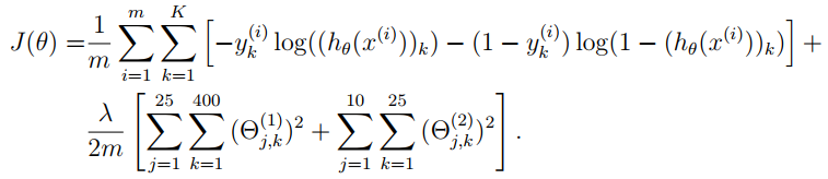
回顧下神經網絡的代價函數(不帶正則化項)
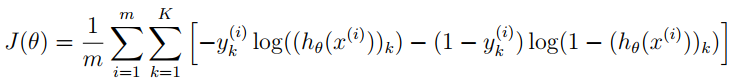
輸出層輸出的是對樣本的預測,包含5000個數據,每個數據對應了一個包含10個元素的向量,代表了結果有10類。在公式中,每個元素與log項對應相乘。
最后我們使用提供訓練好的參數θ,算出的cost應該為0.287629
def cost(theta, X, y):
    a1, z2, a2, z3, h = feed_forward(theta, X)
    J = 0
    for i in range(len(X)):
        first = - y[i] * np.log(h[i])
        second = (1 - y[i]) * np.log(1 - h[i])
        J = J + np.sum(first - second)
    J = J / len(X)
    return J
'''
     # or just use verctorization
     J = - y * np.log(h) - (1 - y) * np.log(1 - h)
     return J.sum() / len(X)
'''
cost(theta, X, y) # 0.2876291651613189
1.4 Regularized cost function 正則化代價函數
注意不要將每層的偏置項正則化。
最后You should see that the cost is about 0.383770
def regularized_cost(theta, X, y, l=1):
    '''正則化時忽略每層的偏置項,也就是參數矩陣的第一列'''
    t1, t2 = deserialize(theta)
    reg = np.sum(t1[:,1:] ** 2) + np.sum(t2[:,1:] ** 2)  # or use np.power(a, 2)
    return l / (2 * len(X)) * reg + cost(theta, X, y)
regularized_cost(theta, X, y, 1) # 0.38376985909092354
2 Backpropagation 反向傳播
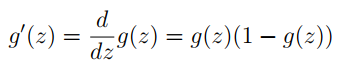
2.1 Sigmoid gradient S函數導數
這里可以手動推導,并不難。
def sigmoid_gradient(z):
    return sigmoid(z) * (1 - sigmoid(z))
2.2 Random initialization 隨機初始化
當我們訓練神經網絡時,隨機初始化參數是很重要的,可以打破數據的對稱性。一個有效的策略是在均勻分布(−e,e)中隨機選擇值,我們可以選擇 e = 0.12 這個范圍的值來確保參數足夠小,使得訓練更有效率。
def random_init(size):
    '''從服從的均勻分布的范圍中隨機返回size大小的值'''
    return np.random.uniform(-0.12, 0.12, size)
2.3 Backpropagation 反向傳播
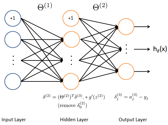
目標:獲取整個網絡代價函數的梯度。以便在優化算法中求解。
這里面一定要理解正向傳播和反向傳播的過程,才能弄清楚各種參數在網絡中的維度,切記。比如手寫出每次傳播的式子。
print('a1', a1.shape,'t1', t1.shape)
print('z2', z2.shape)
print('a2', a2.shape, 't2', t2.shape)
print('z3', z3.shape)
print('a3', h.shape)
'''
a1 (5000, 401) t1 (25, 401)
z2 (5000, 25)
a2 (5000, 26) t2 (10, 26)
z3 (5000, 10)
a3 (5000, 10)
'''
def gradient(theta, X, y):
    '''
    unregularized gradient, notice no d1 since the input layer has no error
    return 所有參數theta的梯度,故梯度D(i)和參數theta(i)同shape,重要。
    '''
    t1, t2 = deserialize(theta)
    a1, z2, a2, z3, h = feed_forward(theta, X)
    d3 = h - y # (5000, 10)
    d2 = d3 @ t2[:,1:] * sigmoid_gradient(z2)  # (5000, 25)
    D2 = d3.T @ a2  # (10, 26)
    D1 = d2.T @ a1 # (25, 401)
    D = (1 / len(X)) * serialize(D1, D2)  # (10285,)
    return D
2.4 Gradient checking 梯度檢測
在你的神經網絡,你是最小化代價函數J(Θ)。執行梯度檢查你的參數,你可以想象展開參數Θ(1)Θ(2)成一個長向量θ。通過這樣做,你能使用以下梯度檢查過程。
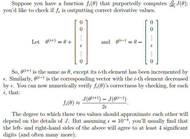
def gradient_checking(theta, X, y, e):
    def a_numeric_grad(plus, minus):
        """
        對每個參數theta_i計算數值梯度,即理論梯度。
        """
        return (regularized_cost(plus, X, y) - regularized_cost(minus, X, y)) / (e * 2)
    numeric_grad = []
    for i in range(len(theta)):
        plus = theta.copy()  # deep copy otherwise you will change the raw theta
        minus = theta.copy()
        plus[i] = plus[i] + e
        minus[i] = minus[i] - e
        grad_i = a_numeric_grad(plus, minus)
        numeric_grad.append(grad_i)
    numeric_grad = np.array(numeric_grad)
    analytic_grad = regularized_gradient(theta, X, y)
    diff = np.linalg.norm(numeric_grad - analytic_grad) / np.linalg.norm(numeric_grad + analytic_grad)
    print('If your backpropagation implementation is correct,\nthe relative difference will be smaller than 10e-9 (assume epsilon=0.0001).\nRelative Difference: {}\n'.format(diff))
gradient_checking(theta, X, y, epsilon= 0.0001)#這個運行很慢,謹慎運行
2.5 Regularized Neural Networks 正則化神經網絡
def regularized_gradient(theta, X, y, l=1):
    """不懲罰偏置單元的參數"""
    a1, z2, a2, z3, h = feed_forward(theta, X)
    D1, D2 = deserialize(gradient(theta, X, y))
    t1[:,0] = 0
    t2[:,0] = 0
    reg_D1 = D1 + (l / len(X)) * t1
    reg_D2 = D2 + (l / len(X)) * t2
    return serialize(reg_D1, reg_D2)
2.6 Learning parameters using fmincg 優化參數
def nn_training(X, y):
    init_theta = random_init(10285)  # 25*401 + 10*26
    res = opt.minimize(fun=regularized_cost,
                       x0=init_theta,
                       args=(X, y, 1),
                       method='TNC',
                       jac=regularized_gradient,
                       options={'maxiter': 400})
    return res
res = nn_training(X, y)#慢
res
'''
     fun: 0.5156784004838036
     jac: array([-2.51032294e-04, -2.11248326e-12,  4.38829369e-13, ...,
        9.88299811e-05, -2.59923586e-03, -8.52351187e-04])
 message: 'Converged (|f_n-f_(n-1)| ~= 0)'
    nfev: 271
     nit: 17
  status: 1
 success: True
       x: array([ 0.58440213, -0.02013683,  0.1118854 , ..., -2.8959637 ,
        1.85893941, -2.78756836])
'''
def accuracy(theta, X, y):
    _, _, _, _, h = feed_forward(res.x, X)
    y_pred = np.argmax(h, axis=1) + 1
    print(classification_report(y, y_pred))
accuracy(res.x, X, raw_y)
'''
             precision    recall  f1-score   support
          1       0.97      0.99      0.98       500
          2       0.98      0.97      0.98       500
          3       0.98      0.95      0.96       500
          4       0.98      0.97      0.97       500
          5       0.97      0.98      0.97       500
          6       0.99      0.98      0.98       500
          7       0.99      0.97      0.98       500
          8       0.96      0.98      0.97       500
          9       0.97      0.98      0.97       500
         10       0.99      0.99      0.99       500
avg / total       0.98      0.98      0.98      5000
'''
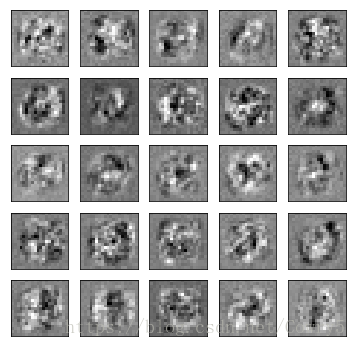
3 Visualizing the hidden layer 可視化隱藏層
理解神經網絡是如何學習的一個很好的辦法是,可視化隱藏層單元所捕獲的內容。通俗的說,給定一個的隱藏層單元,可視化它所計算的內容的方法是找到一個輸入x,x可以激活這個單元(也就是說有一個激活值接近與1)。對于我們所訓練的網絡,注意到θ1中每一行都是一個401維的向量,代表每個隱藏層單元的參數。如果我們忽略偏置項,我們就能得到400維的向量,這個向量代表每個樣本輸入到每個隱層單元的像素的權重。因此可視化的一個方法是,reshape這個400維的向量為(20,20)的圖像然后輸出。
注:
It turns out that this is equivalent to finding the input that gives the highest activation for the hidden unit, given a norm constraint on the input.
這相當于找到了一個輸入,給了隱層單元最高的激活值,給定了一個輸入的標準限制。例如(||x||2≤1)
(這部分暫時不太理解)
def plot_hidden(theta):
    t1, _ = deserialize(theta)
    t1 = t1[:, 1:]
    fig,ax_array = plt.subplots(5, 5, sharex=True, sharey=True, figsize=(6,6))
    for r in range(5):
        for c in range(5):
            ax_array[r, c].matshow(t1[r * 5 + c].reshape(20, 20), cmap='gray_r')
            plt.xticks([])
            plt.yticks([])
    plt.show()
到此在這篇練習中,你將學習如何用反向傳播算法來學習神經網絡的參數,更多相關機器學習,神經網絡內容請搜索腳本之家以前的文章或繼續瀏覽下面的相關文章,希望大家以后多多支持腳本之家!
您可能感興趣的文章:- 吳恩達機器學習練習:SVM支持向量機
- python 機器學習的標準化、歸一化、正則化、離散化和白化
- 利用機器學習預測房價
- 深度學習詳解之初試機器學習
- AI:如何訓練機器學習的模型